What is Featuristic?

Featuristic uses Genetic Algorithms to automate the process of feature engineering and feature selection, enhancing the performance of machine learning models by optimizing their predictive capabilities.

Understanding Genetic Feature Synthesis

Featuristic uses symbolic regression to intelligently derive interpretable mathematical formulas, which are then used to create new features from your dataset.

Initially, Featuristic creates a diverse population of formulas using fundamental mathematical operators such as add, subtract, sin, tan, square, sqrt, and more.

For instance, a formula generated by Featuristic might look like this: (square(feature_1) - abs(feature_2)) * feature_3.

Next, Featuristic assesses the importance of these formulas by quantifying how well they correlate with the target variable. Those formulas yielding features with the strongest correlations are then selected and recombined using a genetic algorithm to produce offspring, as illustrated below.

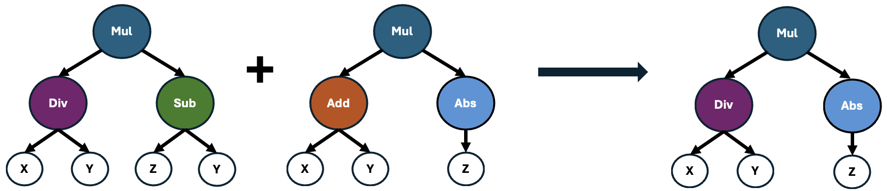
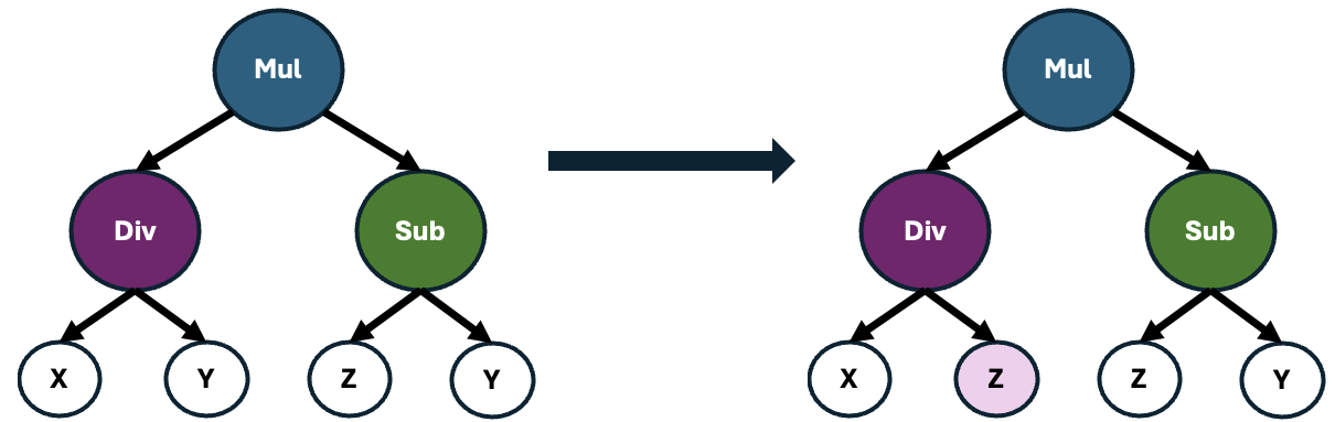
These offspring may also undergo point mutations, which causes alterations to random operators within the formula. This process introduces slight variations to the formulas, enhancing the diversity of the population and potentially leading to the discovery of novel and more effective feature representations.

This iterative process continues across multiple generations, continually refining the population of formulas with the goal of generating features that exhibit strong correlations with the target variable.

Quickstart

Below is a simple example of how Featuristic performs automated feature engineering and selection on the widely used cars dataset.

Featuristic operates in two distinct steps:

1. Genetic Feature Synthesis: In this initial phase, Featuristic intelligently evolves new features through a form of symbolic regression. This involves the generation of mathematical expressions using genetic algorithms. These expressions are designed to capture complex relationships within the dataset.

2. Genetic Feature Selection: Following the creation of new features, Featuristic employs a Genetic Feature Selection algorithm. This algorithm searches through the newly formed feature space to identify the most optimal subset of features. The objective is to maximize predictive accuracy while minimizing the number of features required for model training.

from sklearn.linear_model import LinearRegression
from sklearn.model_selection import train_test_split, cross_val_score
from sklearn.metrics import mean_absolute_error
import featuristic as ft
import numpy as np

np.random.seed(8888)

print(ft.__version__)

1.0.1

Load the Data

X, y = ft.fetch_cars_dataset()

X.head()

	displacement	cylinders	horsepower	weight	acceleration	model_year	origin
0	307.0	8	130.0	3504	12.0	70	1
1	350.0	8	165.0	3693	11.5	70	1
2	318.0	8	150.0	3436	11.0	70	1
3	304.0	8	150.0	3433	12.0	70	1
4	302.0	8	140.0	3449	10.5	70	1

y.head()

0    18.0
1    15.0
2    18.0
3    16.0
4    17.0
Name: mpg, dtype: float64

Genetic Feature Synthesis

Now, let’s dive into the fun part: using Genetic Feature Synthesis to automatically engineer new features from our dataset!

Before we proceed, it’s important to ensure a robust evaluation of our model’s performance. To achieve this, we’ll first split our dataset into training and testing sets. The training set will be used to train our model, while the testing set will remain unseen during the training process and will serve as an independent dataset to evaluate the model’s performance.

Once our data is appropriately split, we’ll initiate the Genetic Feature Synthesis process. We’ve configured the genetic algorithm to synthesize 5 new features for us. This entails evolving a population consisting of 200 individuals iteratively over 100 generations. To ensure optimal performance, we’ve set the genetic algorithm to halt early if it fails to improve upon the best feature identified within 25 generations. Additionally, for enhanced computational efficiency, we’ve designated n_jobs as -1, enabling concurrent execution across all available CPUs on our computer.

With everything set up, we simply call the fit function to generate our new features.

X_train, X_test, y_train, y_test = train_test_split(X, y, test_size=0.33)

synth = ft.GeneticFeatureSynthesis(
    num_features=5,
    population_size=200,
    max_generations=100,
    early_termination_iters=25,
    parsimony_coefficient=0.035,
    n_jobs=-1,
)
synth.fit(X_train, y_train)

None

Creating new features...:  48%|███████▋        | 48/100 [00:19<00:21,  2.43it/s]
Pruning feature space...: 100%|██████████████████| 5/5 [00:00<00:00, 519.75it/s]
Creating new features...:  48%|███████▋        | 48/100 [00:19<00:21,  2.44it/s]

Next, we call the transform function to generate a dataframe containing our new features. By default, the GeneticFeatureSynthesis class will return both the original features and the newly synthesised features. However, we return just the new features by setting the return_all_features argument to False when we create the class.

We can also combine both the fit and transform steps into one step by calling fit_transform instead.

generated_features = synth.transform(X_train)

generated_features.head()

	displacement	cylinders	horsepower	weight	acceleration	model_year	origin	feature_0	feature_4	feature_11	feature_1	feature_22
0	89.0	4	62.0	2050	17.3	81	3	-8571.629032	-0.312535	-96.744944	-105.822581	-0.624987
1	318.0	8	150.0	4077	14.0	72	1	-2488.320000	-0.786564	-75.169811	-34.560000	-1.573022
2	383.0	8	170.0	3563	10.0	70	1	-2017.647059	-0.727317	-71.827676	-28.823529	-1.454460
3	260.0	8	110.0	4060	19.0	77	1	-4150.300000	-0.684937	-82.626923	-53.900000	-1.369706
4	318.0	8	140.0	4080	13.7	78	1	-3389.657143	-0.670713	-81.360377	-43.457143	-1.341324

Our newly engineered features currently have generic names. However, since Featuristic synthesizes these features by the applying mathematical expressions to the data, we can look at the underlying formulas responsible for each feature’s creation.

info = synth.get_feature_info()
info["formula"].iloc[0]

'-(abs((cube(model_year) / horsepower)))'

Feature Selection

Following the synthesis of new features, the next step involves using another genetic algorithm for feature selection. This process sifts through the pool of features to identify the subset that optimally contributes to predictive performance while minimizing redundancy.

Define the Cost Function

We set up a custom objective function that the Genetic Feature Selection algorithm will use to quantify how well the subset of features predicts the target. Please note that the function should return a value to minimize so a smaller value is better. If you want to maximize a metric, you should multiply the output of your objective_function by -1, as shown in the example below.

def objective_function(X, y):
    model = LinearRegression()
    scores = cross_val_score(model, X, y, cv=3, scoring="neg_mean_absolute_error")
    return scores.mean() * -1

Next, we set up the Genetic Feature Selector. We’ve configured the genetic algorithm to evolve a population consisting of 200 individuals iteratively over 100 generations. To ensure optimal performance, we’ve set the genetic algorithm to halt early if it fails to improve upon the best feature set identified within 25 generations. Additionally, for enhanced computational efficiency, we’ve set n_jobs as -1, enabling concurrent execution across all available CPUs on our computer.

selector = ft.GeneticFeatureSelector(
    objective_function,
    population_size=200,
    max_generations=100,
    early_termination_iters=25,
    n_jobs=-1,
)

selector.fit(generated_features, y_train)

selected_features = selector.transform(generated_features)

print(len(selected_features.columns))

Optimising feature selection...:  27%|██▍      | 27/100 [00:05<00:13,  5.34it/s]

8

The Selected Features

Let’s print out the selected features to see what the Genetic Feature Selection algorithm kept. You can see below that featuristic has kept four of the original features (“weight”, “acceleration”, “model_year” and “origin”) plus four of the features created via the Genetic Feature Synthesis.

selected_features.head()

	weight	acceleration	model_year	origin	feature_0	feature_4	feature_11	feature_1
0	2050	17.3	81	3	-8571.629032	-0.312535	-96.744944	-105.822581
1	4077	14.0	72	1	-2488.320000	-0.786564	-75.169811	-34.560000
2	3563	10.0	70	1	-2017.647059	-0.727317	-71.827676	-28.823529
3	4060	19.0	77	1	-4150.300000	-0.684937	-82.626923	-53.900000
4	4080	13.7	78	1	-3389.657143	-0.670713	-81.360377	-43.457143

Training a Model

Now that we’ve selected our features, let’s see whether they actually help our model’s predictive performance on our test data set. We’ll start off with the original features as a baseline.

model = LinearRegression()
model.fit(X_train, y_train)
preds = model.predict(X_test)
original_mae = mean_absolute_error(y_test, preds)
original_mae

2.5888868138669303

And now, let’s see how the model performs with our synthesised feature set.

model = LinearRegression()
model.fit(selected_features, y_train)
test_features = selector.transform(synth.transform(X_test))
preds = model.predict(test_features)
featuristic_mae = mean_absolute_error(y_test, preds)
featuristic_mae

1.9497667311649802

print(f"Original MAE: {original_mae}")
print(f"Featuristic MAE: {featuristic_mae}")
print(f"Improvement: {round((1 - (featuristic_mae / original_mae))* 100, 1)}%")

Original MAE: 2.5888868138669303
Featuristic MAE: 1.9497667311649802
Improvement: 24.7%

The new features generated / selected by the Genetic Feature Synthesis have successfully reduced our mean absolute error 😀

Table of Contents

• Installation
• Guides
• Examples

Resources & References

• Release Notes
• API Reference

Other Links

• Index

• Search Page